Dynamic Models of Human Systems

Introduction: An Overview of Dynamic System Models

(PDF version)

Models in Science

According to Merriam-Webster, a model, among other things, is “a description or analogy used to help visualize something (such as an atom) that cannot be directly observed, or “a system of postulates, data, and inferences presented as a mathematical description of an entity or state of affairs,” and also, “a computer simulation based on such a system.”

Models are, rather purposefully, not reality; rather they are simplified abstractions of reality that scientists create to help them understand and explore the key features of complex phenomena. They are similar to laboratory experiments in which most of the real world is controlled away in order to focus on a select few processes. Models in science are refined over time to make them useful for improving understanding, exploring new possibilities, or making predictions. If models end up not being useful, they are simply discarded or, perhaps more accurately, fade away as their proponents retire.

Sometimes, the models that scientists devise are, literally, physical models, a classic example being the 1953 model of a DNA molecule constructed by Francis Crick and James Watson—a glorified Tinker Toy model. More often, models are verbal; a written, simplified description of some aspect of reality. Verbal models, if they cover a broad area of science and become widely accepted, are referred to as theories. A classic example of a verbal model is Darwin’s evolutionary theory as described in his On the Origins of Species. Verbal models are sometimes accompanied by visual diagrams—a picture being worth (on occasion) a thousand words.

Watson (left) and Crick and their physical model of the DNA molecule.

Many scientific models are mathematical—equations or sets of equations that describe the behavior of some physical, biological, or social phenomena. Mathematical models can be created to match, at least approximately, past observations and, if they are good models, to predict future behavior with reasonable accuracy. Mathematical models are also useful for checking the cogency of verbal theories. Words are imprecise and mathematical models based on verbal theories often lead to unexpected results.

For example, Darwin thought that biological inheritance was the blending of parental traits. However, a mathematical critic pointed out that blending inheritance averages away the variation that Darwin’s theory of natural selection required to work, exposing a major problem with Darwin’s verbal theory. The problem was partially solved in the early 20^th Century by the discovery that genes are discrete units that do not blend. Understanding how heritable variation is preserved is, to this day, still an important topic in evolutionary biology.

In recent decades, scientists have increasingly employed computer models as tools for schooling their intuitions and for explaining, exploring, and predicting. While computer models can simply implement mathematical models—making them more convenient and less labor-intensive to use—they can also include non-mathematical features unique to computer programing.

The social sciences—which include anthropology, philosophy, economics, history, political science, psychology, and sociology—study extraordinarily complex systems. Similar to physical and biological scientists, social scientists construct non-mathematical models to help them understand and explore the essence of humanity. Until recently, many social scientists and humanists thought that human behavior was too complex to be “reduced” to mathematical models. They still make less use of mathematical models than natural scientists.

Yet even the very simplest natural science systems can, in essence, only be completely reduced to mathematical models. In some cases, like turbulent motions in air and water, the phenomenon of interest can be reduced to a model, but the model will still be so complex that it is extremely difficult to analyze. This is also the case with social systems, which are much more complex than turbulent motion. In principle we might reduce a social system to a model, but it would be so complex that it would be impossible to analyze. With modern computers you can simulate rather complex systems, but the resulting simulations are very hard to understand. Substituting a model you don’t understand for a real world you don’t understand is not progress!

It turns out, however, that relatively simple mathematical approximations of complex dynamic systems do prove to be important tools for explanation, exploration, and prediction. Mathematical modelers often say, “All models are wrong, but some models are useful.” The data available about complex social systems is often rather limited compared to their real-world complexity. Nevertheless, if we think of models as hypotheses about what are the dominant processes at work in a complex system, then testing hypotheses boils down to fitting competing models to data and selecting the best fitting model as the currently most useful one.

This is trickier than it sounds because data is always more or less heavily contaminated with error. If you fit a too complex model, you will fit the error as well as the underlying processes you want to understand. Practically speaking, you can only aspire to successfully fit rather simple models to systems we know in principle are much more complex. Often, all the most useful model can do is tell us which dominant process or two was operating over the span of time covered by the data. Paradoxically, simple models are often useful because they tell us all that we can practically know about a complex system.

Verbal models can say a lot about a complex system but only rather imprecisely. Mathematical models usually say less but with greater precision. Verbal and mathematical models are thus complementary approaches to studying complex dynamic systems.

Wise scientists and managers are cautious around complex systems. It is easy to talk yourself into believing you know more than you do really do about them! The imprecision of your verbal model can haunt you. Your most useful quantitative model can come undone if a formerly minor driver of the system becomes a major one, a not infrequent occurrence. A manager of a complex system is a little like a circus lion tamer. No matter how well you know your cat, she is still a wild, dangerous beast that can surprise you.

Another way to think about it is that models are like airplanes, microscopes, and telescopes. Humans can’t fly and our eyes can’t resolve very small or very distant objects. The human mind is not particularly good at quantitative reasoning and computes rather slowly. Formal math and computer simulations are devices that help us get around this limitation.

Systems

A “system,” according to Merriam-Webster, is “a regularly interacting or interdependent group of items forming a unified whole.” A system is delineated by establishing a boundary that defines what is within the system and what is outside. Many systems can be modeled as a process or mechanism that, over time, transform inputs into outputs; inputs are utilized to produce outputs.

The outputs of a static system depend only on the current inputs to the system, not on earlier inputs. The outputs of dynamic systems, on the other hand, depend not only on current inputs but also on past inputs, thus allowing for delayed system responses. This “feedback,” of past performance effecting future performance can produce, even for simple dynamic systems, quite unexpected, complex, and even counter-intuitive results.

Models of Dynamic Systems

Isaac Newton, Gottfried Wilhelm Leibniz, and Joseph-Louis Lagrange were the first to model physical dynamic systems (starting with astronomical orbits) using differential equations. A differential equation is a mathematical relationship between functions (variables) and their derivatives. Derivatives are rates of change, often with respect to time. For instance, if the distance one has driven down a road in miles is a variable, then its derivative is the rate of distance change, which is speed (miles per hour). Since the initial modeling of simple physical systems, differential equations (both single equations and sets of two or more linked equations) have provided useful mathematical models of chemical, biological, and (recently) human dynamic systems.

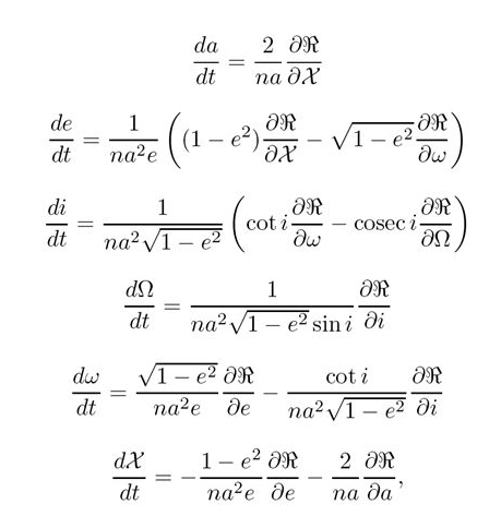
Lagrange’s differential equations model of planetary motion.

The behavior of a complex system can be explored if the system can be described by a set of equations or, alternatively, a computer program that provides a set of rules that, given the current state of the system, projects what the state of the system (and its outputs) will be a small step of time in the future. This new system state, and the same fixed rules, are then used to calculate the next state of the system. This recursive process is simply repeated over and over; this way the model works its way from some initial starting point forward, off into the future, one little time step at a time. A bit like an inch worm.

Classical calculus assumes that each time step is infinitely small. This enables mathematicians to deploy some wonderful analytical tricks as long as the model is rather simple. Methods devised to be implemented on digital computers can handle more complex models. They use finite time steps that feed the results from calculations at the last time step back into the underlying transformational rules to obtain the results for the next time step. These calculations are typically repeated for many tiny time steps (hundreds, thousands, or more) to map out the behavior of the model system through time. Large, fast computers can implement more complex models and take more, smaller steps. The ongoing quest for ever bigger and faster computers is driven, in part, by the practical needs of certain models. For instance, models used for weather prediction and understanding the evolution of the climate are limited by the power of current computers. Predicting the future performance of economies is another practical problem with a lot of similarities to weather prediction.

Given a set of fixed rules, these rules will determine the unique output the modeled system will produce, off into the future, given any particular initial conditions at the start time (t = 0) and the value of the parameters (coefficients) applied to the rules. If you run the same model again, with the same initial conditions and model parameters, you will always get the same identical result. That is, unless you deliberately introduce random variation into your model or unless your system includes the possibility of chaotic dynamics!

One explores the behavior of the modeled system by exercising or “running” the model. The model is often devised as a set of differential equations, initial conditions are set (such as an initial human population), model parameters are adjusted (such as birth rate and death rate), and Run is clicked. The model, one small increment of time after the other, applies the rules to calculate the outputs over time (such as total population, year-by-year for a century). This is called “running the model,” or a “simulation.”

In the days before digital computers, human computers had to run the models. Tedious calculations had to be made over and over again for each little step in time; and this was for just one set of initial conditions and set of model parameters. The result was that it simply was impractical, before the advent of digital computers, to explore the “landscape” of most dynamic models. Thus their counterintuitive, oftentimes strange behaviors remained hidden. The pioneering meteorologist Lewis F. Richardson took a year or so during World War I, using hand calculations, to calculate the changes the weather would make in six real hours. His basic modeling methods are now calculated with digital computers in minutes, forecasting the weather for days ahead with reasonably accuracy.

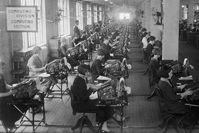
Before there were digital computers, running a simulation model took a roomful of mechanical calculators and human operators to calculate all the points on the output curves.

There is no reason, of course, given the same initial conditions and model parameters, to run a model more than once (assuming the model does not have random statistical elements). There is every reason, however, to run the model many times while changing the initial conditions and/or the values of the model parameters (independent variables) each time the model is run. How does the system behavior change (i.e. how do the outputs vary over time) as the initial conditions and model parameters are varied?

Answering this question can be difficult even for fairly simple models. Consider a model with three initial conditions and three model parameters. If each of these can be set to one of 10 values, then the combination of these, if one wanted to explore all the possibilities, would be astronomical; yet, a major reason for constructing such models is to explore all potentially interesting possibilities. This phenomenon is sometimes called “the curse of dimensionality.”

For any given system, one can typically set a range of values one might reasonably expect for each initial condition and model parameter. One can then change each parameter by a small amount (say 1% of the range) to get a feel for how sensitive the model behavior is to this particular parameter. If it is not sensitive, then just leave it alone and don’t worry about it. On the other hand, if it is sensitive, then it is an important parameter that should be changed to explore its effect. This sensitivity analysis is an important aspect of system analysis. Modelers try to follow the KISS Rule, “Keep it simple stupid.” Or, paraphrasing Einstein, modelers often say “Models should be as simple as possible, but no simpler.”

If a relatively simple dynamic system had only two inputs (x and y) and one output (z), the results of running the system with all the combinations of the two inputs would produce an x-y-z “landscape.” For instance, consider the case where x = population, y = resource consumption, and z = planetary health. By fine tuning the two input parameters (x and y), one can figure out how to climb to the top of a peak of planetary health (z), but unless one has tried all the x/y combinations, one could never be sure there isn’t a higher, as yet unclimbed, peak somewhere else in the landscape. Clever schemes have been devised to be reasonably sure you found all the peaks without literally trying every x/y combination.

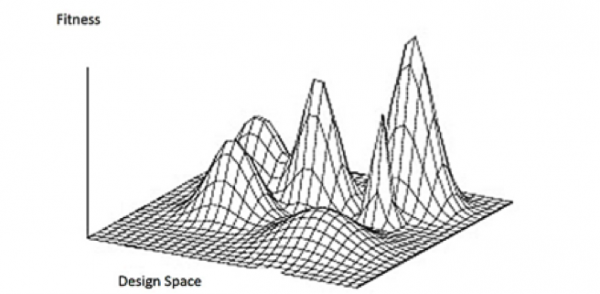
Dynamic x-y-z landscape. One can climb a peak easily enough, but it is more difficult to know whether or not you have climbed to the top of the highest peak.

The Behavior of Dynamic Systems Models

Many systems models, if you let them run long enough, either stop changing over time and hence become “steady state,” or they eventually “blow up” as some key parameter heads toward infinity. In the simple population model mentioned earlier, if death rates exceed birth rates, eventually everyone dies, and the population drops to zero and stays there, a steady state outcome. On the other hand, if the birth rate exceeds the death rate, then sooner or later the population will take off and head toward infinity, blowing up the model.

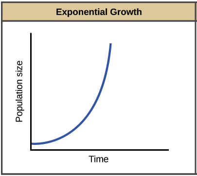
In an exponential population growth model, the population heads toward infinity as time progresses.

There is an interesting case where the birth rate exactly equals the death rate. In this special case the model population will stay at its initial value as time goes on, essentially forever.

The case where the population goes to zero or some other invariant value is a final, “dynamically stable,” “steady-state” case represented by the ball on the left, while the case where the birth and death rates are exactly equal is a “dynamically unstable” state represented by the ball on the right. The least change in rates will eventually send the population to zero (or the model could blow up as the population heads toward infinity). However, if we make a bit more complex model, the population can go to a finite stable carrying capacity equilibrium.

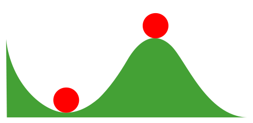
Some systems (balls) are dynamically stable (ball on the left) while others are unstable (ball on the right).

In the real world, there are many dynamically unstable systems where we do not want things to either go to zero or blow up, and yet a relatively small change could send things off in one catastrophic direction or another. To keep things “balanced” near the unstable point we need to actively adjust the system parameters as time goes by to avoid having the system head off toward disaster. This is sometimes termed adaptive management. Our climate, at least with runaway human technology in the mix, may have become somewhat unstable. A relatively small change in atmospheric CO2 concentrations could cause a small rise in temperature, which melts snow and ice, making the planet less reflective thus absorbing even more heat, which melts even more snow and ice … you get the idea.

Using Dynamic Models for Guidance

Dynamic models can help guide us as to which system parameters we should consider adjusting. Usually it is best to adjust the more impactful (sensitive) parameters, as there is no sense wasting efforts trying to change things that have little if any overall effect on the system. Even more critically, dynamic system models can help inform us in which direction we should change a sensitive parameter to achieve the desired result.

One would think that the direction the change needed to be made should be obvious but, as mentioned previously, the performances of dynamic systems are often counterintuitive. When you adjust a system parameter in some direction, hoping to move the system back to some desired state, it may, much to your surprise, make things worse, not better. If you had, instead, made the adjustment in the counterintuitive direction, things would have improved. For example, people tend to think that providing monetary rewards or punishments will increase desired behaviors. But sometimes the effect of monetary incentives is to encourage people to think that some behavior is not a moral issue but rather just a matter of money. A small fine, that violators can easily afford to pay, for bad behavior may thus encourage bad behavior! Models can be useful guides to which changes might be the most helpful to make and in what direction the changes should be made.

It might be noted that models do not have to be very accurate or complex to provide vital information on which parameters are sensitive and which direction sensitive parameters should be adjusted to move a system in the desired direction. However, they function in an important way that non-dynamic models (such as verbal models or “linear” models) do not. Such models often provide little information on which parameters are most impactful and, worse yet, they often suggest corrective changes be made in the wrong (but intuitive) direction. The bottom line: humans, unaided, do not have an intuitive feel for many (even most) dynamic systems, and most important systems are dynamic.

Rabbits and Foxes Scenario

Internally, dynamic models often have positive or negative feedback loops. Positive feedbacks tend to make things increase more and more over time, moving a model toward an infinity blowup. Negative feedbacks tend to make changes decrease as time goes by, heading the model toward some steady state, often zero.

Many real-world cases involve dynamic systems with both positive and negative feedbacks. Positive feedback speeds up change, but then negative feedback can kick in full force and slow change down. Continuously going up and down over time, the dynamic system oscillates. A swinging pendulum or vibrating string are classic examples of physically oscillating systems.

The classic biological example of an oscillating system is the rabbits-and-foxes scenario. Pretend that our model world starts out on a big, remotely located island covered with luscious green grass but otherwise deserted. We introduce an initial population of 200 rabbits and set their birth rate higher than their death rate (after all these are rabbits). Then we click the Run button and the rabbits start eating the grass. Soon there are lots of little bunnies and the rabbit population zooms upward toward infinity as the island heads toward ecological collapse. Wishing to stave off such an undesirable outcome, we hurriedly hit the Stop button on our model and devise a new model.

Our new model, along with the same initial population of 200 rabbits, introduces foxes, also with an initial population of 200. We click the Run button. This time, the foxes go wild and eat most of the rabbits. Lots of little foxes are born as the rabbit population plunges. Soon rabbits are scarce and hard to find. The foxes starve and their population drops. At some point there are not many foxes around to eat the rabbits and so, again, the rabbit population booms. Back and forth it goes over time, first lots of foxes and then lots of rabbits, an oscillating future until the end of time, a sea-level rise submerges the island, or we get bored and hit the Stop button, whichever comes first.

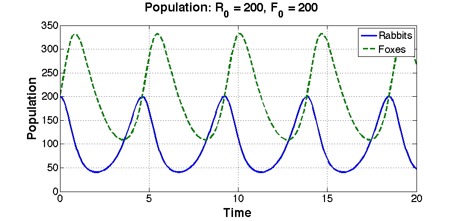
Foxes (dashed line) multiply as they eat all those yummy rabbits, while the rabbit population plummets. Then after most of the foxes starve to death, the rabbit population rebounds. On and on …

White Box Models

While all the models we will describe in this course are based on differential equations, you will not need to know or learn anything about differential equations to understand and use the models or, for that matter, to devise your own models as a follow-on exercise after you finish this course. The reason for this is that these models can be laid out visually as block diagrams with inputs and outputs, positive and negative feedback loops, etc. A block diagram is a diagram of a system in which the key parts or functions are represented by blocks or other shapes that are connected by lines with arrows that show relationships. Once the model is laid out visually in the graphics-enabled computer program (described below), the computer program itself converts the diagram into one or more differential equations; it is not necessary to understand the mathematics or do any computer programming since it is all visual.

Understanding the inner workings of a model by way of a visual diagram is a helpful but not an absolute prerequisite for using a model. While one can use (drive) a car without learning what is “under the hood,” at least a summary (block diagram) knowledge of the engine, drive train, and other mechanical features of the car will make you a better-informed driver.

Models are sometimes thought of as being contained in a box. If the box (model) can be opened to see what is inside, it is termed a “white box.” If you are not allowed to see inside it is called a “black box.” In this course we will first consider models as white boxes, allowing you to look under the hood before you jump in to drive the models. Once in the driver’s seat the models will be treated as black boxes, just showing you the controls and a display of the results from running the model, your out-the-window view of where you went with your model.

White box models are different than black box models because you can open them up and see what is inside.

It should be noted that the visual block diagram models are just as complete as the differential equation models. They are, in fact, just a different representation of the same thing. We provide, as an aside, the differential equations for each model so if mathematical equations appeal to you more than visual block diagrams, you can just ignore the latter. To provide a bridge between the visual and mathematical models, parameter names are spelled out in the block model along with their abbreviated symbols and mathematical equations.

Black Box Models

You can, as suggested above, run the models without knowing what is inside the model—even as a visual block diagram, let alone a set of differential equations. When you do this, you are running the model as a “black box.” A black box is a scientific, computational, or engineering name for a system or device that can be viewed just in terms of its inputs and outputs without any knowledge of its internal workings, which could be extraordinarily complex. Because the user cannot see what is inside the black box—because it is opaque or has been blacked out—it is called a black box.

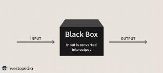
With a black box model, you can see just the inputs and outputs. All the complexities of the model are hidden inside of the black (opaque) box.

In this course we will run each of our models from a black box perspective. We provide the inputs you are allowed to make (set initial conditions and adjust system parameters); then you click the Run button. The black-box model shows how outputs (like rabbit and fox populations) change over time.

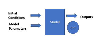
A slightly refined version of a black box model.

We can then change our inputs and run our model again and see how changing the inputs changes the outputs. If we experiment around with the model enough, we can draw some conclusions about how the model behaves and, to the extent that the model represents the real world, and what we might expect to happen if we changed things in the real world. The key point is that we can learn a lot about how models behave (and even how the real world might behave) by playing around with black box models. We do not have to know what is inside the box to get a good feel for the often-counterintuitive behavior of dynamic (as opposed to linear) systems. Sometimes it is best not to get distracted with the details. You may enjoy sausage more if you do not visit the sausage factory.

To run a model, set the initial conditions, adjust the model parameters to desired values, and then click the Run button. The model will then take small steps through time, computing and graphing your outputs as it goes. That is all there is to it. This allows concentrated learning about dynamic systems, including some hands-on experience with a number of examples drawn from the social sciences.

Computer Programs for Visual Dynamic Models

There are two popular computer programs that are used to visually construct dynamic systems using block diagrams and, once constructed, run (simulate) the model to explore its dynamic responses. One program is Vensim and the other is Stella. Vensim, developed by Ventana Systems, is an open-source (free) program somewhat similar to Stella. While not as visually attractive and easy to use as Stella, it is widely used at universities. Both are descendants of DYNAMO (DYNAmic MOdels) that was developed by Phyllis Fox while working for Jay Forrester at MIT in the late 1950s. Forrester was a pioneer in developing digital computers and also the field of system dynamics via computer simulations.

Stella, originally all capitalized as STELLA (short for Systems Thinking, Experiential Learning Laboratory with Animation), was developed by Barry Richmond and has been in use in various versions since 1985. It is currently available from isee systems. The online Stella models used in the units in this course are free, as is an online, web-based isee systems software you can use to construct your own simple models. While the full-featured software to build complex models is not free, it is available at low cost to high school students and teachers and is easy to use.

The Stella models used in this course were devised using Stella Architect. They can be run, online, at no cost, and they do not require any user software—just bring the model up online, set the initial conditions and system parameters as desired for a run, and click Run. Your results will be displayed. The visual block diagrams, which we provide with each dynamic model that we have developed for you, are relatively straight forward and easy to understand, should you choose to explore them.

Barry Richmond’s book, An Introduction to Systems Thinking, is both an explanation of the use and function of Stella modeling and a rich exploration of the “Thinking, Communicating, and Learning” processes that underlay model building logic. Richmond’s book also identifies eight invaluable systems thinking skills that guide effective use of modeling processes; Richmond believes these skills have significant educational value. If you would like to explore these ideas further, an overview graphic and summary narrative of the model building processes and the development of systems thinking skills—Dynamic Systems Thinking and Modeling—is provided after the last model. The systems thinking skills are particularly easy to grasp and can be a considerable aid in academic and professional endeavors, as well as everyday critical thinking about the world around us.

Conclusion

The whole point of modeling, as suggested by Meadows (1999) in the title of one of her papers, is to find Leverage Points: Places to Intervene in a System. Leverage points, as she suggests, “are places within a complex system where a small shift in one thing can produce big changes in everything.” The problem, as Meadows suggests, is that “leverage points are not intuitive. Or if they are, we intuitively use them backwards [moving system parameters in the wrong direction], systematically worsening whatever problems we are trying to solve.”

The hope is that dynamic system models, such as you will be studying, will illuminate our situation, suggest key leverage points to influence, and the correct direction they should be nudged. This course will introduce you to the dynamic systems point of view. The tools you learn to use will help you appreciate complex situations in the social sciences, be on the alert for potential counterintuitive behavior, look for those key leverage points, and consider how they might be nudged in the right direction to improve our social systems and humanity’s interaction with other species and the planet.

Aside from such “think big” questions, dynamic models, such those as you will learn about, are used to study and manage a host of smaller scale applied problems including weather forecasting, economic forecasting, demographic projections, fish and game management, endangered species protection, and the management of epidemics. They have, so far, barely tapped potential in fields like applied sociology and international relations, not to mention in the basic sciences that underpin the applied ones.

---

Further Reading

A review of some important work on modeling of the kind we use in this module:

Efferson, C. and P. J. Richerson (2007). A prolegomenon to non-linear empiricism in the human sciences. Biology and Philosophy 22(1): 1-33. [Link]

Essays advocating the approach we use in this module:

Richerson, P. J. and R. Boyd (1998). Homage to Malthus, Ricardo, and Boserup: Toward a general theory of population, economic growth, environmental deterioration, wealth, and poverty. Human Ecology Review 4:85-90. [Link]

Waring, T. M. and P. J. Richerson (2011). Towards unification of the socio-ecological sciences: the value of coupled models. Geografiska Annaler: Series B, Human Geography 93(4): 301-314. [Link]

Detailed introduction to the important Russian school of socio-economic modeling:

Korotayev, A., A. Malkov and D. Khalttourina (2006). Introduction to Social Macrodynamics: Secular cycles and millennial trends. Moscow, Editorial URSS. [Link]

Textbook on Lotka-Volterra style models:

Brauer, F. and C. Castillo-Chavez (2012). Mathematical Models in Population Biology and Epidemiology, Springer.

Top of page

---